ggplot2: How Geoms & Aesthetics ≈ Whipped Cream

In this post I have a few goals:

1. Become (re-)familiar with available geoms
2. Become (re-)familiar with aesthetic mappings in geoms (stroke who knew?)
3. Answer these questions:

• How often do various geoms appear and how often do they have required aesthetics?
• How often do various aesthetics appear and how often are they required?
• What geoms are most similar based on mappings?

The Back Story

Two weeks go I made whipped cream for the first time. In a tweet I lamented not having tried making it earlier in my life:

This was an error that resulted in missing out because of a lack of confidence. Now the opposite tale. Missing out because of false confidence. I know ggplot2…there’s nothing new to learn. Recently I realized it’s been too long since I’ve re-read the documentation. I’m betting my time making this blog post that there’s a few more like me.

I’m teaching an upcoming analysis course.  To prepare I’m reading and rereading many important texts including R for Data Science.  In my close read I noticed that some ggplot2 functions have a stroke aesthetic.

Didn’t know that…I figure I needed to spend a bit more time with the documentation and really get to know geoms and aesthetics that I may have overlooked. 

What’s an aesthetic Anyways?

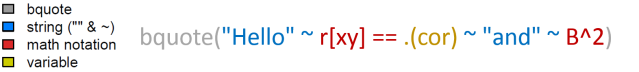
ggplot2’s author, Hadley, states:

In brief, the grammar tells us that a statistical graphic is a mapping from data to aesthetic attributes (colour, shape, size) of geometric objects (points, lines, bars)….aesthetics…are the properties that can be perceived on the graphic. Each aesthetic can be mapped to a variable, or set to a constant value.  pp. 4; 176

So without aesthetics, geoms can’t represent data.

Getting the Geoms and Their Aesthetics

Before getting started note that wordpress.com destroys code. To get the undestroyed version of code from this blog use this gist: https://gist.github.com/trinker/a03c24a7fe9603d3091f183ffe4781ab

I wasn’t sure how I was going to accomplish this task but a little digging showed that it was pretty easy.  First I used Dason Kurkiewicz  & I’s pacman package to get all the geoms from ggplot2.  This is where I first hit a road block.  How do I get the aesthetics for a geom?  I recalled that the documentation tells you the aesthetics for each geom.  I noticed that in the roxygen2 markup the following line that creates the aesthetics reference in the documentation:

@eval rd_aesthetics("geom", "bar")

That allowed me to follow the bread crumbs to make the following code to grab the aesthetics per geom and a flag for when an aesthetic is required:

if (!require("pacman")) install.packages("pacman")
pacman::p_load(pacman, ggplot2, dplyr, textshape, numform, tidyr, lsa, viridis)

## get the geoms
geoms <- gsub('^geom_', '', grep('^geom_', p_funs(ggplot2), value = TRUE))

## function to grab the aesthetics
get_aesthetics <- function(name, type){

    obj <- switch(type, geom = ggplot2:::find_subclass("Geom", name, globalenv()), 
        stat = ggplot2:::find_subclass("Stat", name, globalenv()))
    aes <- ggplot2:::rd_aesthetics_item(obj)

    req <- obj$required_aes

    data_frame(
        aesthetic = union(req, sort(obj$aesthetics())),
        required = aesthetic %in% req,

    )
}

## loop through and grab the aesthetics per geom
aesthetics_list <- lapply(geoms, function(name){

    type <- 'geom'
 
    name <- switch(name,
        jitter = 'point',
        freqpoly = 'line',
        histogram = 'bar',
        name
    )

    out <- try(get_aesthetics(name, 'geom'), silent = TRUE)

    if (inherits(out, 'try-error')) out %
    setNames(geoms)

## convert the list of data.frames to one tidy data.frame
aesthetics %
    tidy_list('geom') %>%
    tbl_df()

aesthetics

   geom   aesthetic required
             
 1 abline slope     TRUE    
 2 abline intercept TRUE    
 3 abline alpha     FALSE   
 4 abline colour    FALSE   
 5 abline group     FALSE   
 6 abline linetype  FALSE   
 7 abline size      FALSE   
 8 area   x         TRUE    
 9 area   y         TRUE    
10 area   alpha     FALSE   
# ... with 341 more rows

Geoms: Getting Acquainted

First I wanted to get to know geoms again. There are currently 44 of them.

length(unique(aesthetics$geom))

## 44

This bar plot details the geoms and how many aesthetics are optional/required.

geom_ord %
    count(geom) %>%
    arrange(n) %>%
    pull(geom)


aesthetics %>%
    mutate(geom = factor(geom, levels = geom_ord)) %>%
    ggplot(aes(geom, fill = required)) +
        geom_bar() +
        coord_flip() +
        scale_y_continuous(expand = c(0, 0), limits = c(0, 15)) +
        scale_fill_manual(name = 'Required', values = c('gray88', '#1C86EE'), labels = f_response) +
        theme_minimal() +
        theme(
            panel.grid.major.y = element_blank(),
            axis.text = element_text(color = 'grey55', size = 10),
            legend.key.size = unit(.35, 'cm'),
            legend.title = element_text(color = 'grey30', size = 10),
            legend.position = c(.76, .1),
            axis.title = element_text(color = 'gray55')
        ) +
        labs(
            x = 'Geom',
            y = 'Count',
            title = 'Count of Geom Aesthetics',
            subtitle = 'Distribution of geom aesthetic count filled by requirement flag.'

        ) 

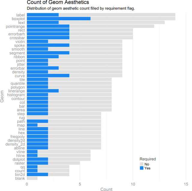
Some interesting things come out. Most geoms have 2ish required aesthetics. The boxplot geom has the most required and unrequired aesthetics. Sensibly, a blank geom requires no aesthetics. I wanted to see what all of these aesthetics were for the boxplot. Some quick dplyr-ing has us there in no time.

aesthetics %>%
    filter(geom == 'boxplot')

   geom    aesthetic required
              
 1 boxplot x         TRUE    
 2 boxplot lower     TRUE    
 3 boxplot upper     TRUE    
 4 boxplot middle    TRUE    
 5 boxplot ymin      TRUE    
 6 boxplot ymax      TRUE    
 7 boxplot alpha     FALSE   
 8 boxplot colour    FALSE   
 9 boxplot fill      FALSE   
10 boxplot group     FALSE   
11 boxplot linetype  FALSE   
12 boxplot shape     FALSE   
13 boxplot size      FALSE   
14 boxplot weight    FALSE   

Seems that x is the only aesthetic that is truly required. The other “required” ones are computed if you just supply x.

Aesthetics: May I join You?

Now time to get to know aesthetics. Are there others like stroke that I’ve overlooked? There are 36 aesthetics currently. I see right away that there is a weight aesthetic I’ve never seen before.

length(unique(aesthetics$aesthetic))

## 36

aes_ord %
    count(aesthetic) %>%
    arrange(n) %>%
    pull(aesthetic)

aesthetics %>%
    mutate(aesthetic = factor(aesthetic, levels = aes_ord)) %>%
    ggplot(aes(aesthetic, fill = required)) +
        geom_bar() +
        scale_y_continuous(expand = c(0, 0), limits = c(0, 45), breaks = seq(0, 45, by = 5)) +
        scale_fill_manual(name = 'Required', values = c('gray88', '#1C86EE'), labels = f_response) +
        theme_minimal() +
        theme(
            panel.grid.major.y = element_blank(),
            panel.grid.minor = element_blank(),
            axis.text = element_text(color = 'grey55', size = 10),
            legend.key.size = unit(.35, 'cm'),
            legend.title = element_text(color = 'grey30', size = 10),
            legend.position = c(.83, .1),
            axis.title = element_text(color = 'gray55')
        ) +
        labs(
            x = 'Aesthetic',
            y = 'Count',
            title = 'Count of Aesthetics',
            subtitle = 'Distribution of aesthetics filled by requirement flag.'
        ) +
        coord_flip()

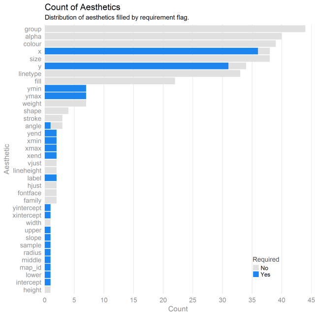
It seems from this plot that almost every geom requires an x/y position aesthetic. That makes sense. What doesn’t make sense are cases besides geom_blank that don’t require x/y.

aesthetics %>%
    filter(aesthetic %in% c('x', 'y') & !required)

  geom  aesthetic required
           
1 count y         FALSE   
2 qq    x         FALSE   
3 qq    y         FALSE   
4 rug   x         FALSE   
5 rug   y         FALSE 

This dplyr summarize/filter shows where an x/y are possible aesthetics but not required. Sensible. But are there some geoms that x/y aren’t even in their mapping?

aesthetics %>%
    group_by(geom) %>% 
    summarize(
        has_x = 'x' %in% aesthetic, 
        has_y = 'y' %in% aesthetic 
    ) %>%
    filter(!has_x | ! has_y) %>%
    arrange(has_x)

   geom      has_x has_y
         
 1 abline    FALSE FALSE
 2 blank     FALSE FALSE
 3 hline     FALSE FALSE
 4 map       FALSE FALSE
 5 rect      FALSE FALSE
 6 vline     FALSE FALSE
 7 boxplot   TRUE  FALSE
 8 errorbar  TRUE  FALSE
 9 linerange TRUE  FALSE
10 ribbon    TRUE  FALSE

Dig into the documentation if you want to make sense of why these geoms don’t require x/y positions.

Geoms & Aesthetics Intersect

OK so we’ve explored variability in geoms and aesthetics a bit…let’s see how they covary. The heatmap below provides an understanding of what geoms utilize what aesthetics and if they are required. NA means that the aesthetic is not a part of the geom’s mapping.

boolean %
    count(geom, aesthetic) %>%
    spread(aesthetic, n, fill = 0)


boolean %>%
    gather(aesthetic, value, -geom) %>%
    left_join(aesthetics, by  = c('geom', 'aesthetic')) %>%
    mutate(
        aesthetic = factor(aesthetic, levels = rev(aes_ord)),
        geom = factor(geom, levels = rev(geom_ord))        
    ) %>%
    ggplot(aes(y = aesthetic, x = geom, fill = required)) +
         geom_tile(color = 'grey95') +
         scale_fill_manual(name = 'Required', values = c('gray88', '#1C86EE'), labels = f_response) +
         theme_minimal() +
         theme(
             axis.ticks = element_blank(),
             axis.text.y = element_text(size = 8, margin = margin(r = -3)),
             axis.text.x = element_text(size = 8, hjust = 1, vjust = 1, 
                 angle = 45, margin = margin(t = -3)),   
             legend.key.size = unit(.35, 'cm'),
             legend.title = element_text(color = 'grey30', size = 10),
             panel.grid = element_blank(),
             axis.title = element_text(color = 'gray55')                
         ) +
         labs(
             title = 'Geom & Aesthetic Co-occurrence',
             subtitle = NULL, 
             y = 'Aesthetic',
             x = 'Geom'
         )

Here we can see that weight aesthetic again. Hmmm, boxplot has it and other, mostly univariate functions as well. The documentation is a bit sparse on it. Hadley says: https://github.com/tidyverse/ggplot2/issues/1893

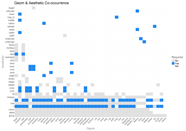
Also there are two geoms that are just now catching my eye…geom_count & geom_spoke. I’ll come back to them later.

Also, there are a few aesthetics like height and intercept that are one time use only aesthetics. Also, the bottom 10 aesthetics are used, by far, the most frequently. For beginners, these are the ones that will really pay to learn quickly.

Geom Similarity

I thought it my be fun to use the geoms aesthetics to see if we could cluster aesthetically similar geoms closer together. The heatmap below uses cosine similarity and heirarchical clustering to reorder the matrix that will allow for like geoms to be found closer to one another (note that today I learned from “R for Data Science” about the seriation package [https://cran.r-project.org/web/packages/seriation/index.html] that may make this matrix reordering task much easier).

boolean %>%
    column_to_rownames() %>% 
    as.matrix() %>%
    t() %>%
    cosine() %>%
    cluster_matrix() %>%
    tidy_matrix('geom', 'geom2') %>%
    mutate(
        geom = factor(geom, levels = unique(geom)),
        geom2 = factor(geom2, levels = unique(geom2))        
    ) %>%
    group_by(geom) %>%
    ggplot(aes(geom, geom2, fill = value)) +
         geom_tile() +
         scale_fill_viridis(name = bquote(cos(theta))) +
         theme(
             axis.text.y = element_text(size = 8)   ,
             axis.text.x = element_text(size = 8, hjust = 1, vjust = 1, angle = 45),   
             legend.position = 'bottom',
             legend.key.height = grid::unit(.2, 'cm'),
             legend.key.width = grid::unit(.7, 'cm'),
             axis.title = element_text(color = 'gray55')               
         ) +
         labs(
             title = "ggplot2 Geom Cosine Similarity",
             subtitle = 'Geoms with similar aesthetics are clustered together along the diagonal.',
             x = 'Geom',
             y = 'Geom'
         )

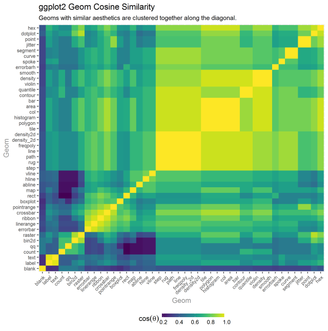
Looking at the bright square clusters along the diagonal is a good starting place for understanding which geoms tend to aesthetically cluster together. Generally, this ordering seems pretty reasonable.

Aesthetic Similarity

I performed the same analysis of aesthetics, asking which ones tended to be used within the same geoms.

boolean %>%
    column_to_rownames() %>% 
    as.matrix() %>%
    cosine() %>% 
    {x <- .; diag(x) %
    cluster_matrix() %>%
    tidy_matrix('aesthetic', 'aesthetic2') %>%
    mutate(
        aesthetic = factor(aesthetic, levels = unique(aesthetic)),
        aesthetic2 = factor(aesthetic2, levels = unique(aesthetic2))        
    ) %>%
    group_by(aesthetic) %>%
    ggplot(aes(aesthetic, aesthetic2, fill = value)) +
         geom_tile() +
         scale_fill_viridis(name = bquote(cos(theta))) +
         theme(
             axis.text.y = element_text(size = 8)   ,
             axis.text.x = element_text(size = 8, hjust = 1, vjust = 1, angle = 45),   
             legend.position = 'bottom',
             legend.key.height = grid::unit(.2, 'cm'),
             legend.key.width = grid::unit(.7, 'cm'),
             axis.title = element_text(color = 'gray55')                
         ) +
         labs(
             title = "ggplot2 Aesthetics Cosine Similarity",
             subtitle = f_wrap(c(
                 'Aesthetics that tend to be used together within the same geoms are clustered together along the diagonal.'
                 ), width = 95, collapse = TRUE
             ), 
             x = 'Aesthetic',
             y = 'Aesthetic'
         )

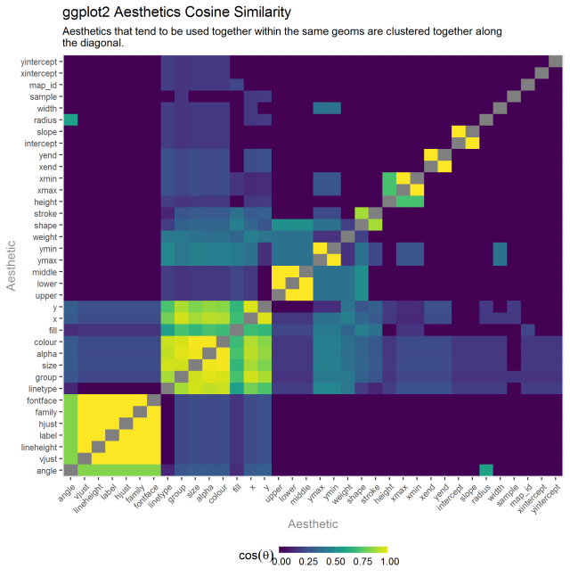
The result is pretty sensible. The lower left corner has the largest cluster which seems to be related to text based geoms. The next cluster up and to the right one, has group, size, x, y, etc. This seems to be the most common set of typically geometric aesthetics. The upper, lower, middle cluster is specific to the boxplot summary stat. Stroke and shape as a cluster are related to geoms that are point based.

Geom Similarity: Required Aesthetics

The last clustering activity I wanted was to reduce the seahetics to jsut required (as we might assume these are the truest attributes of a geom) and see which geoms cluster from that analysis.

boolean2 %
    filter(required) %>%
    count(geom, aesthetic) %>%
    spread(aesthetic, n, fill = 0)

	
boolean2 %>%
    column_to_rownames() %>% 
    as.matrix() %>%
    t() %>%
    cosine() %>%
    cluster_matrix() %>%

    tidy_matrix('geom', 'geom2') %>%
    mutate(
        geom = factor(geom, levels = unique(geom)),
        geom2 = factor(geom2, levels = unique(geom2))        
    ) %>%
    group_by(geom) %>%
    ggplot(aes(geom, geom2, fill = value)) +
         geom_tile() +
         scale_fill_viridis(name = bquote(cos(theta))) +
         theme(
             axis.text.y = element_text(size = 8)   ,
             axis.text.x = element_text(size = 8, hjust = 1, vjust = 1, angle = 45),   
             legend.position = 'bottom',
             legend.key.height = grid::unit(.2, 'cm'),
             legend.key.width = grid::unit(.7, 'cm'),
             axis.title = element_text(color = 'gray55')                
         ) +
         labs(
             title = "ggplot2 Geom Cosine Similarity",
             subtitle = 'Geoms with similar aesthetics are clustered together along the diagonal.',
             x = 'Geom',
             y = 'Geom'
         )

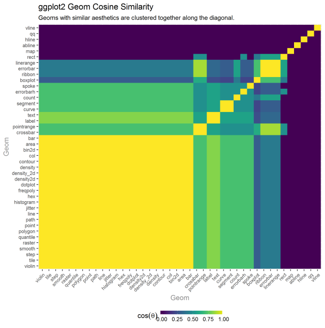
This seemed less interesting. I didn’t really have a plausible explanation for what patterns did show up and for the most part, clusters became really large or really small. I’m open to others’ interpretations.

A Few Un-/Re-discovered ggplot2 Features

I did want to learn more about geom_count & geom_spoke in the remaining exploration.

?geom_count

ggplot(diamonds, aes(x = cut, y = clarity)) + 
    geom_count(aes(size = ..prop.., group = 1)) +
    scale_size_area(max_size = 10)

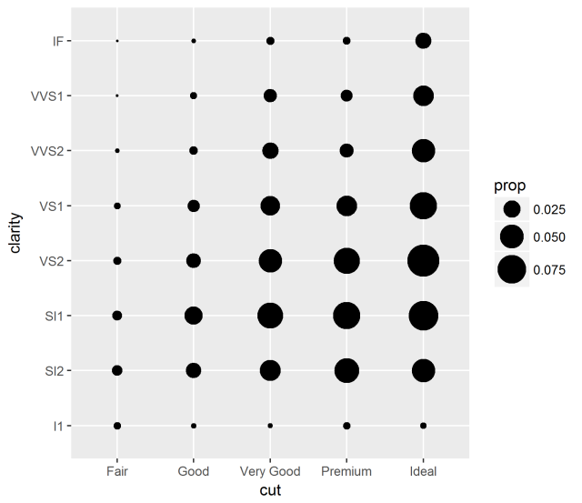
Oh yeah! Now I remember. A shortcut to make the geom_point bubble plot for investigating categorical variable covariance as an alternative to the heatmap.

?geom_spoke

df <- expand.grid(x = 1:10, y=1:10)
df$angle <- runif(100, 0, 2*pi)
df$speed <- runif(100, 0, sqrt(0.1 * df$x))

ggplot(df, aes(x, y)) +
    geom_point() +
    geom_spoke(aes(angle = angle), radius = 0.5)

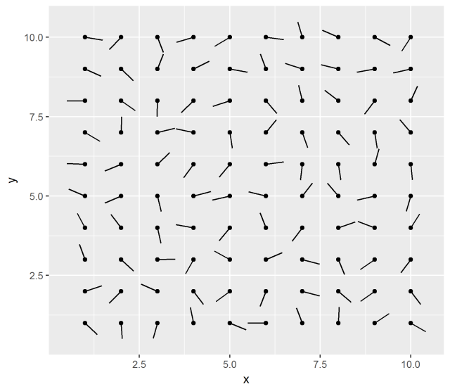
Interesting. The documentation says:

…useful when you have variables that describe direction and distance.

Not sure if I have a use case for my own work. But I’ll store it in the vault (but better than I remembered geom_count).

Learning More About Geoms & Aesthetics

I wanted to leave people with a quick reference guide that RStudio has kindly provided to help give quick reference to geoms and aesthetics and whe to use them.

Math Notation for R Plot Titles: expression, bquote, & Greek Letters

In this post you will learn:

1. How to create expressions that have mixed (1) strings, (2) expressions, (3) variables & (4) Greek letters
2. How to pass in values as variables to an expression

I wanted to name this post “Ahhhhhhhhhhh #$@%&!!!!” but SEO isn’t terrific for this title so I tried to make the actual title as Googleable as possible. I’m writing this post for future me and past me. If some of the rest of you find it useful even better.

Problem: Math Expressions
Specifically: Plotting Them

Seems every-time I need to plot a title with math notation I wind up wasting a half an hour on what ought to be an easy task.  It’s probably because I don’t have the need to do this task often.  It’s also because R has it’s own way to write maths (not LaTeX or something I’m familiar with).  It is also because there’s several ways to accomplish this task in R.  It’s also because I’ve never spent the time defining how to do the process.  I  can only control the latter two of these four.  Today I define how to write a plot with a title that has a math expression.

Success is if I can easily plot the following title:

This is a layperson’s guide written for and by a layperson.  I’m sure there’s a precise reason for what and why plotting math notations is quirky.  I don’t have the cognitive space or care to know why.  I’m learning and sharing enough to reliably get the job done.  In the future maybe I’ll care more about the why.

Math Notations Require an Expression or Call

This was my first aha.  I don’t know exactly what an expression or call is.  I also don’t know if math notation can be done without these but since I’m focused on a single way to get this don’t let’s just go with this for now.  I just know it’s not a string for sure.  Hadley has a whole chapter on expressions if you really want the full treatment read about it here:  http://adv-r.had.co.nz/Expressions.html  I’ve read it a few times but my brain hasn’t retained the distinctions long-term yet. This stackoverflow question also explains a great bit of the detail between an expression and a call: https://stackoverflow.com/q/20355547/1000343  But let’s get back to the task at hand…a single way to plot the above title with mixed strings, notation, & numbers.

Use bquote

I’ve seen mixed string, number, and math expression annotation done with expression, parse(text=, bquote, substitute & clever use of back ticks. For me, the most straight forward way is bquote. It seems to be pretty flexible for most tasks. Here are the four rules to overcome math notation title blues when using bquote:

1. Strings – Require quotes wrapped w/ tilde separator (e.g., "my text"  ~).
2. Math Expressions – Unquoted & follow ?plotmath
3. Numbers – Unquoted when part of math notation
4. Variables – Use .() (pass in string or numeric)

Got that? Great!

Application

Now you can build what ever.  For example say we want to (1) pass a variable name to a plot title, (2) followed by a math notation (correlation), (3) being equal to a correlation value, (4) followed by a string, and lastly, (5) one more math notation. Well that’s:

Use the rules.   Here’s a visual representation of the rules.  Notice that only a string gets quotes around it?  Notice the tilde separators around quoted strings?  Notice the cor value is passed in (more on this in a moment)?  If you struggle with the math notation see ?plotmath

Note that if the correlation being passed in as a variable were just a number manually placed in the expression the value is simply part of the math notation.

Example

Code:

I’m going to plot this 2 times.  One where the variable cor being passed in is a double and then a string (cor2).  Notice that the leading zero is used in the double?

## A variable to pass in
cor <- -.321
cor2 <- '-.321'

par(mfrow = c(1, 2))
plot(1:10, 1:10, main = bquote("Hello" ~ r[xy] == .(cor) ~ "and" ~ B^2))
plot(1:10, 1:10, main = bquote("Hello" ~ r[xy] == .(cor2) ~ "and" ~ B^2))

Results in:

ggplot2: Me To!

Works for ggplot2 as well.

library(ggplot2)

ggplot() + labs(title = bquote("Hello" ~ r[xy] == .(cor2) ~ "and" ~ B^2))

Another Way

Alas there is more than one way to accomplish math notation in titles in R.  If you want one way then bquote and the 4 rules will likely always get it done.  Skip this brief section.

If you’re still reading…You can also use a parse(text = and paste method.  The two approaches are similar to a sprintf vs. paste approach to string manipulation (see paste, paste0, and sprintf).  This approach requires a bit more reasoning and the cor2 is coerced to a double with a leading zero when it’s evaluate?

There are more ways too but I’ll leave that for the curious reader 🙂
 

plot(1:10, 1:10, main = parse(text = paste0('"Hello"', ' ~ r[xy] == ', cor2, '~ B^2')))

Hopefully, this post helps me in the future to understand how to format plot titles that contain math notation.  I hope it helps you too.  Note that this thinking is generalizable to other plot annotations with math notations besides titles. Also, I came across this nicely formatted overview of plotmath and wanted to share: http://vis.supstat.com/2013/04/mathematical-annotation-in-r

Addendum: Greek Letters

As a follow up Julia Silge asked about Greek letters. I hadn’t included them in this post but future me and others will likely be concerned about these puppies as well.

I hadn’t tried Greek letters with the bquote approach so I decided to try it with a regression line equation as seen below. Thankfully, bquote seems to work here too.

cor2 <- '-.321'

plot(
    1:10, 
	1:10, 
	main = bquote("Eq 1:" ~ y[i] == alpha + beta * x[i] + epsilon[i] ~ "or" ~ .(cor2))
)

## And ggplot2 as well
library(ggplot2)

ggplot() + 
    labs(title = bquote("Eq 1:" ~ y[i] == alpha + beta * x[i] + epsilon[i] ~ "or" ~ .(cor2)))

Using R to Reason & Test Theory: A Case Study from the Field of Reading Education

Note: Word Press messes up the code. Find the code here: https://github.com/trinker/RandomCaseEffect

This past week I was preparing slides for a reading assessment class with a lecture focus on the Visual Word Form Area [VWFA] (Cohen, et al., 2000). This is an area of the brain that is hypothesized to be able to see words (plus morphemes and likely smaller chunks) as shapes, as picture forms and that may have a connecting link between the visual and language portions of the brain.

In a sense it allows a proficient reader to see words and know them in the same way that we see people’s faces and we know them (if we’ve encountered them before). Essentially, phonics is useful, particularly at certain points in our reading development but is rather inefficient and not the work horse of a proficient reader’s reading process. Instant word recognition is required for fluency and comprehension. For additional information on the reading process see the video below.

Cohen, L., Dehaene, S., Naccache, L., Lehéricy, S., Dehaene-Lambertz, G., Hénaff, M. A., Michel, F. (2000). The visual word form area: Spatial and temporal characterization of an initial stage of reading in normal subjects and posterior split-brain patients. Brain. 123(2). 291–307. doi:10.1093/brain/123.2.291. ISSN 0006-8950. PMID 10648437

As I prepared for class I wanted to demonstrate two points about the VWFA to students:

1. General shape of words is an attribute used by the VWFA
2. The first and last letter are very important to instant word recognition; the exact ordering of the individual letters (graphemes) of the middle portions of words less important

The first can be evidenced by altering the case of letters within words and seeing it does indeed slow down reading rate. The second can be demonstrated by randomly reordering the inner letters within a word. The amount of case changing or reordering of letters are parameters that can be changed and can slow down reading rate in varied ways. What better way to demonstrate this than using R to reason and programatically allow the testing of theory. The two sections below show R code that tests the (1) altering case theory of the VWFA and (2) the lowered importance of the ordering of the middle letters of words.

First you’ll need to install my textshape package to get started:

if (!require("pacman")) install.packages("pacman"); library(pacman)
pacman::p_load(textshape)

Altering Case Effects

Mayall, Humphreys & Olson (1997) show that letter case randomization can disrupt the ability to process words. If true, this is evidence that the VWFA (if it exists) uses a general shape attribute for word recognition since mixing case alters shape not letters.

Mayall, K., Humphreys, G. W., & Olson, A. (1997). Disruption to word or letter processing?: The origins of case-mixing effects. Journal of Experimental Psychology: Learning, Memory, and Cognition, 23(5), 1275-1286. 10.1037/0278-7393.23.5.1275

The R script below is a function that takes text and randomly replaces a set proportion of lower case letters with upper case. In the script below I show some text that has 2%, 10%, and 50% (worst case; no pun intended) of lower case letters randomly replaced with upper case letters. The reader can informally see that indeed the letters are the same but the picture quality seen by the brain reduces the ability to process the words. Secondly, 2% change is less disruptive than 50%. This is evidence that there is a VWFA and one of the attributes it uses is word shape.

#' Randomly Change the Case of Letters Within Words
#' 
#' Following Mayall, Humphreys, & Olson (1997), this function randomly 
#' converts a proportion of lower case letters to upper case.
#' 
#' @param x A vector of text strings to upper case.
#' @param prop A proportion of graphemes to change the case of.
#' @param wrap An integer value of how wide to wrap the strings.  Using the default 
#' \code{NULL} disables this feature.
#' @param \ldots ignored.
#' @return Prints wrapped lines with internal graphemes randomly converted to 
#' upper case.
#' @references 
#' Mayall, K., Humphreys, G. W., & Olson, A. (1997). Disruption to word or letter 
#' processing?: The origins of case-mixing effects. Journal of Experimental Psychology: 
#' Learning, Memory, and Cognition, 23(5), 1275-1286. 10.1037/0278-7393.23.5.1275
#' @export
random_upper  0 & prop <= 1)

    ## splits each string to a vector of characters
    char_vects <- strsplit(x, '')

    ## loop through each vector of characters and replace lower with upper case
    out <- unlist(lapply(char_vects, function(chars){

        ## detect the lower case locations
        locs <- grepl('[a-z]', chars)   
        ilocs <- which(locs) 

        ## sample lower case locations to convert to upper 
        to_upper <- sample(ilocs, ceiling(prop * length(ilocs)))  
        chars[to_upper] <- toupper(chars[to_upper])

        ## collapse the vector of characters back to its original string
        paste(chars, collapse = '')

    }))

    ## optional string wrapping
    if (!is.null(wrap) && !is.na(as.integer(wrap))) {
        invisible(Map(function(x, wrapchar) {
            cat(strwrap(x, width = as.integer(wrap)), sep = '\n')
            if (wrapchar) cat('\n')
        }, out, c(rep(TRUE, length(out) - 1), FALSE)))
    } else {
        out
    }

}


x <- "Many English words are formed by taking basic words and adding combinations of prefixes and suffixes to them."

## 2% random upper
random_upper(x, .02, 60)

## MAny English words Are formed by taking basic words and
## adding combinations of prefixes and suffixes to them.

## 30% random upper
random_upper(x, .3, 60)

## Many English words are forMed by taking basic worDs aNd
## adding Combinations of prEFixes and SuffIxeS to them.

## 50% random upper
random_upper(x, .5, 60)

## MaNy EnglIsH WORDs ARE FoRmED BY taking BAsic WOrDs And
## AddiNg CombinATIoNS OF pRefIXEs AnD sUffIXES to thEM.

Transposing Internal Letters

Another interesting phenomenon is the transposing of letters within the middle of words. This was popularized as an Internet meme & hoax about research at Cambridge University:

While the claim the meme makes about the research and Cambridge wasn’t true, obviously, there is an element of truth to the inner word transpose effect noted by researchers in the 70s and 80s (e.g., McCusker, Gough, & Bias, 1981). Indeed the reader can still understand the message but there is a cognitive cost to scrambling letters (Rayner, White, Johnson, & Liversedge, 2006).

McCusker, L. X., Gough, P. B., & Bias, R. G. (1981). Word recognition inside out and outside in. Journal Of Experimental Psychology: Human Perception And Performance, 7(3), 538-551. doi:10.1037/0096-1523.7.3.538

Rayner, K., White, S. J., Johnson, R. L., & Liversedge, S. P. (2006). Raeding wrods with jubmled lettres: There is a cost. Psychological Science, 17(3), 192-193. 10.1111/j.1467-9280.2006.01684.x

The R code below allows the user to group the inner portion of words as character ngrams, reorder within these grams, and optionally reorder the position of the reordered ngram groups. Both the size of the ngrams and the reordering of ngram group position are parameters of the effect that we can alter and informally observe via our self reported effects in our ability to read the strings after altering various parameters. The larger the ngram unit the more the inner portion of words will be scrambled.

The sample.grams parameter allows us to see the effect of keeping scrambled ngram groups in their original position or not. Indeed the longer words are, and the more thorough the remix, the bigger the cost of the letter transpose is. When commonly (or expected) co-occurring ngrams are located randomly (far away from each other) this also may contribute to the cost on scrambling effect. In the final code chunk I allow the first and/or the last letter of words to be scrambled as well. This is evidence that the VWFA is keyed in on the first and last letters and that certain letters are expected to be close to one another.

#' Transpose Internal Letters Within Words
#' 
#' Following a famous Internet meme and Rayner, White, Johnson, & Liversedge 
#' (2006), this function randomly scrambles the internal (not the first or last
#' letter of > 3 character words) letters.
#' 
#' @details Internet meme:
#' 
#' It deosn't mttaer in waht oredr the ltteers in a wrod are, the olny iprmoetnt 
#' tihng is taht the frist and lsat ltteer be at the rghit pclae. The rset can be 
#' a toatl mses and you can sitll raed it wouthit porbelm. Tihs is bcuseae the 
#' huamn mnid deos not raed ervey lteter by istlef, but the wrod as a wlohe.
#'
#' @param x A vector of text strings to scramble.
#' @param gram.length The length of gram groups to scramble.  Setting this lower
#' will keep expected graphemes close together.  Setting it to a high value (e.g.,
#' 100) will allow the positions of graphemes to deviate farther from the expected
#' clustering.
#' @param sample.grams logical.  If \code{TRUE} then the ngram groups don't retain
#' their original location.  For example, let's say we had the sequence \code{123456}. 
#' Sampling grams of length 3 (\code{gram.length} may produce \code{231564}. Setting 
#' \code{sample.grams = TRUE} may further produce \code{564231}.
#' @param wrap An integer value of how wide to wrap the strings.  Using the default 
#' \code{NULL} disables this feature.
#' @param remix.first logical.  If \code{TRUE} the first letter is allowed to be 
#' remixed as well.
#' @param remix.last logical.  If \code{TRUE} the last letter is allowed to be 
#' remixed as well.
#' @param \ldots ignored.
#' @return Prints wrapped lines with internal graphemes scrambled.
#' @references 
#' Rayner, K., White, S. J., Johnson, R. L., & Liversedge, S. P. (2006). Raeding 
#' wrods with jubmled lettres: There is a cost. Psychological Science, 17(3), 
#' 192-193. 10.1111/j.1467-9280.2006.01684.x
#' @export
random_scramble <- function(x, gram.length = 2, sample.grams = TRUE, wrap = NULL, 
    remix.first = FALSE, remix.last = FALSE, ...){

    if (!is.integer(gram.length)) gram.length  1))

    ## splits the strings into a list of tokens (words and punctuation)
    token_vects <- textshape::split_token(x, lower = FALSE)

    ## loop through the vectors of tokens
    out <- unlist(lapply(token_vects, function(tokens){

        ## loop through the tokens within each vector
        out  1) win <- sample(gram.length, 1) else win  3 because you can't transpose words less than 2 internal characters 
            ##   Note: the value of 3 depends if the first and last letters are allowed to vary
            len <- nchar(token)
            if (len < 4 - (remix.first + remix.last)) return(token)

            ## split tokens into characters and compute location of internal letters
            chars <- strsplit(token, '')[[1]]
            locs <- (2 - remix.first):(len - (!remix.last))

            ## If the length of the internal letters is <= the ngram window randomly 
            ##   sample internal letters, collapse characters, and return
            if (length(locs) <= win) {
                return(
                    paste(
                        c(
                            if (remix.first) '' else chars[1], 
                            paste(sample(chars[locs]), collapse = ''), 
                            if (remix.last) '' else chars[length(chars)]
                        ), 
                        collapse = ''
                    )
                )
            }

            ## Make gram groupings for all grams that match gram.length 
            ##    (exclude < gram.length char groups)
            locs2 <- rep(1:floor(length(locs)/win), each = win)

            ## add in the < gram.length groups and store as list of lengths 
            ##    and group assignments 
            locs3 <- rle(c(locs2, c(rep(max(locs2) + 1, length(locs)%%win))))

            ## Resample the lengths to allow the odd group out (if there is one)
            ##     to be located randomly rather than always at the end
            locs4 <- rep(locs3$values, sample(locs3$lengths))

            ## split the vector of chars into the groups, loop through, sample 
            ##     within each group to scramble and collapse the group characters
            rands <- unlist(lapply(split(locs, locs4), function(grams){
                paste(sample(chars[grams]), collapse = '')
            }))

            ## optionally scramble the group location as well
            if (sample.grams) rands <- sample(rands)

            ## collapse the group gram strings together
            paste(
                c(
                    if (remix.first) '' else chars[1], 
                    rands, 
                    if (remix.last) '' else chars[length(chars)]
                ), 
                collapse = ''
            )  

        }))

        ## Paste tokens back together with single space and attmpt to strip out 
        ##     inappropriate spaces before punctuation.  This does not guarentee
        ##     original spacing of the strings.
        trimws(gsub("(\\s+)([.!?,;:])", "\\2", paste(out, collapse = ' '), perl = TRUE))

    }))


    ## optional string wrapping
    if (!is.null(wrap) && !is.na(as.integer(wrap))) {
        invisible(Map(function(x, wrapchar) {
            cat(strwrap(x, width = as.integer(wrap)), sep = '\n')
            if (wrapchar) cat('\n')
        }, out, c(rep(TRUE, length(out) - 1), FALSE)))
    } else {
        out
    }

}

# example text from: https://www.mrc-cbu.cam.ac.uk/personal/matt.davis/Cmabrigde/
x <- c(
    "According to a study at an English University, it doesn't matter in what order the letters in a word are, the only important thing is that the first and last letter be at the right place. The rest can be a total mess and you can still read it without problem. This is because the human mind does not read every letter by itself but the word as a whole.",
    "A vehicle exploded at a police checkpoint near the UN headquarters in Baghdad on Monday killing the bomber and an Iraqi police officer",
    "Big council tax increases this year have squeezed the incomes of many pensioners",
    "A doctor has admitted the manslaughter of a teenage cancer patient who died after a hospital drug blunder."
)

## Bigram & retain mixed ngram group locations
random_scramble(x, gram.length = 2, wrap = 70)

## Aroccnidg to a sduty at an Esngilh Uevrstiniy, it deosn't mteatr in
## what order the ltteers in a word are, the only ipmantrot tnihg is
## that the first and lsat letetr be at the rghit place. The rset can be
## a tatol mses and you can stlil read it wuoihtt pbleorm. Tihs is
## becuase the hamun mnid does not raed eevry lteetr by itself but the
## word as a whole.
## 
## A vehicle exploedd at a polcie cinheckopt naer the UN hrtaueaerdqs in
## Baghadd on Monady kilnlig the bomber and an Iaqri police oceffir
## 
## Big cncouil tax iescnreas tihs yaer hvae sezeequd the iecnmos of mnay
## pneerisons
## 
## A docotr has aitmdetd the mhgtenalsuar of a teegane cnacer pneitat
## who died aetfr a hiptaosl durg bulednr.

## Bigram and reorder the mixed ngram groups
random_scramble(x, gram.length = 2, sample.grams = FALSE, wrap = 70)

## According to a sutdy at an Enlgish Univesrity, it deosn't matetr in
## waht order the lteters in a word are, the olny impotrant thing is
## that the first and last letter be at the right plcae. The rset can be
## a toatl mess and you can still read it wihtuot problem. Tihs is
## because the hmuan mnid deos not raed eevry letetr by istlef but the
## wrod as a whole.
## 
## A vehilce epxoledd at a police checkponit near the UN haedquarters in
## Bgahdad on Monady killing the bmoebr and an Iraqi polcie officer
## 
## Big council tax icnreases this yaer have suqeezed the incoems of mnay
## penisonres
## 
## A dcootr has amditetd the mnaslaughetr of a tenegae cnacer ptaeint
## who deid afetr a hosipatl drug blunder.

## Gram length randomly between 2-5 retain mixed ngram group locations
random_scramble(x, gram.length = 2:5, wrap = 70)

## Accroindg to a sdtuy at an Esilgnh Unveisirty, it d'onset mtetar in
## waht oerdr the lerttes in a wrod are, the only iantormpt tihng is
## taht the frist and last lteetr be at the rhigt plcae. The rset can be
## a taotl mess and you can stlil read it wtuioht pelrobm. This is
## bacusee the haumn mnid deos not raed eervy letter by ieltsf but the
## wrod as a wolhe.
## 
## A viclhee eplodxed at a picloe conikpehct near the UN huaqdearters in
## Bgadhad on Mnoady kililng the bbemor and an Iqari picole ofefcir
## 
## Big cionucl tax ieeascnrs this year hvae seqeuezd the imeocns of mnay
## pnseiorens
## 
## A dotocr has atedmitd the mslautenahgr of a tgaenee cecanr ptianet
## who died after a hatspiol drug bdnelur.

## 5-gram retain mixed ngram group locations
random_scramble(x, gram.length = 5, wrap = 70)

## Accdnirog to a sdtuy at an Elisgnh Usrietnivy, it dnsoe't matetr in
## what oerdr the lrettes in a word are, the olny ianmrotpt tinhg is
## taht the frist and lsat leettr be at the rghit pcale. The rset can be
## a ttoal mses and you can sitll read it woutiht peborlm. Tihs is
## bceause the hmaun mind does not read evrey letetr by ilstef but the
## word as a wolhe.
## 
## A vichlee exolpedd at a piolce conkipehct near the UN hrtearuqdeas in
## Bhagdad on Mndoay knliilg the boembr and an Iqrai poicle ofceifr
## 
## Big cniuocl tax iseenracs this year have seeuqzed the ioncems of mnay
## pernsoines
## 
## A docotr has atemtidd the mlsaanheugtr of a tgeenae canecr pteinat
## who died afetr a haptoisl durg beunldr.

let's ramp it up a bit more and see the effect when we allow the first and last letter to be remixed as well.

## Bigram & retain fixed ngram group locations & remix last letter
random_scramble(x, wrap = 70, remix.last = TRUE)

## Angdiorcc to a sutyd at an Elignsh Uityinsrev, it dns'toe mretta in
## wtha oerrd teh lteters in a wdro aer, teh olny iorpmntat tngih is
## ttah teh frist adn ltsa lertte be at teh rgiht plaec. The rset can be
## a ttoal mses and yuo can sllti rdea it withotu porlbme. Tihs is
## bceesau the hnaum mdin dsoe nto rdae eveyr lttree by ilftse but teh
## wdro as a wohel.
## 
## A velheci eedlodxp at a piloce chekctnipo nera teh UN heartqdrsaue in
## Bgaaddh on Modnay klingil teh berbom and an Iraiq pcieol ociffre
## 
## Big cliuocn txa incasrese tsih yare heva sezqeued the iesomnc of mnya
## pissnoneer
## 
## A dotroc has aittmdde the merhtnagusla of a teeegan cancre patient
## who ddie after a hitspoal durg berlund.

## Bigram & retain fixed ngram group locations & remix first letter
random_scramble(x, wrap = 70, remix.first = TRUE)

## drinoccAg to a tsduy at an Ensiglh inUverstiy, it esod'nt tetamr in
## waht roder the reletts in a rowd are, hte lony rtminapot thing is
## that hte rsift and last eelttr be at hte ghrit aclpe. hTe rest can be
## a taotl sems and oyu acn still eard it thouwit obrpelm. hiTs is
## ebacuse hte uhamn mind deos ont eard ervey etletr by itself but the
## owrd as a hwloe.
## 
## A hievcle olpxeded at a cilpoe nicepkohct aenr hte UN adtrehaureqs in
## daBaghd on ndaoMy kiinllg the bbemor and an aqIri polcie ofcefir
## 
## iBg ocuncil tax eainrcess ihts eyar vahe ezsqueed hte ocinmes of namy
## isprenoens
## 
## A dootcr has tdamited hte utelaamhgnsr of a gaentee caecnr entiapt
## who died teafr a taiphosl urdg deblunr.

## Bigram & retain fixed ngram group locations & remix first + last letters
random_scramble(x, wrap = 70, remix.first = TRUE, remix.last = TRUE) 

## Acicongdr to a yduts ta na Enlihsg tysiivUnre, it t'nsoed amtter ni
## what redro the terstel ni a owrd rae, the noly aimtroptn htign is
## htat the trsif dna stla tterel be ta eht igthr pleca. ehT erts cna eb
## a latot mess nad yuo nca illst daer it wihttuo mprleob. hTis si
## aubcese the hunam mind does otn ader every eltter by tiesfl but eht
## word sa a hwole.
## 
## A ehvleci pldoxede ta a poilce ecntoikpch arne eht UN daehsrrauqte ni
## hdagBda on yaMond illking the rebmbo and na Iqiar poliec ofrecfi
## 
## gBi unocilc txa niesscrae thsi arey have zedeueqs het nimocse fo amyn
## peiorssnne
## 
## A roctod sah adimedtt the ugerlasnmaht fo a teeneag cncare patietn
## how ided etafr a hospitla gudr rnuedbl.

## 5-gram & retain fixed ngram group locations & remix first + last letters
random_scramble(x, wrap = 70, gram.length = 5, remix.first = TRUE, remix.last = TRUE) 

## dingrccoA to a duyst ta na gEinlsh nievUsrity, ti denso't meratt in
## twha drreo the rtestle in a owrd aer, eht ynol nattmiopr tgnhi is
## atth eth isfrt nad salt rtlete be at het trghi claep. Teh tser nac be
## a tlota mses nda ouy nac ltsli read ti witothu rpleobm. Tish si
## ebseuac teh hmaun imdn sdoe otn edra reeyv tetelr by tsilef but hte
## owdr as a ewohl.
## 
## A lehviec epxdldeo ta a oplcie toipnehkcc nrae eth NU auqhedaesrrt ni
## dahgdBa no Mandoy lnlgiki het rombbe dna na rqaIi pcolie ofciefr
## 
## gBi lnciuco txa eassencir tish raey ehav zdeeeqsu hte comnise fo mayn
## osnerniesp
## 
## A doctro hsa edttmdia teh resmnlaathug fo a tneaege cancer nettipa
## woh eddi fatre a hosipatl rdug blnerdu.

This post showed how I recently used R for some quick theory testing and demonstration. Of course the code could be optimized but the point is quick exploration of concepts I'm reading in the literature.

Similar, quick, iterative, testing with R could be done by researchers/teachers across many fields. The field of visualization comes to mind. This could be made into a shiny app to allow non-technical users to still interact with the code. It is my hope that both the content and code is of interest.

Minimal, Explicit, Python Style Package Loading for R

About a year and a half back I was working in Python a bit and became accustomed to the explicit importing of modules (akin to R packages) and functions. Python imports packages like this:

import tidyr
import dplyr as dp
from plyr import l_ply, rbind.fill


If these R packages were in Python, the first line imports tidyr, the second imports dplyr as an object aliased as dp. These 2 lines are how Python imports packages. The user still needs to explicitly prefix objects from these modules when calling them. For example one might call: tidyr.separate or dplyr.select. The third line is more akin to how R loads packages and has access to all exported functions. Still, in Python the user has to explicitly name all functions that are imported. The way that Python imports packages and functions is explicit and may seem annoying to an R user but it avoids NAMESPACE clashes.

Back then I made a proof of concept package called pysty (Python style) to make R behave a bit more like Python for importing packages and functions. I had forgotten about this package…Fast forward to this week.

Within the last 2 days I have been bit by a bug with MASS/dplyr select and a team-mate by plyr/dplyr summarise clashes. I tend to prefix a lot of my functions with their package name now in my code to avoid such headaches. This habit reminded me of pysty. I thought others may find it interesting.

The aliasing makes it convenient to explicitly reference a package without typing out the entire package name when you call it. pysty uses the colon operator to accomplish this explicit calling of functions. Most functions can be imported and added to the global name space in one fell swoop using the from call. All of these Python style calls are possible via the add_imports.

Installing pysty

Let’s start by installing and loading dependencies.

if (!require("pacman")) install.packages("pacman")
pacman::p_load_current_gh('trinker/pysty')

library(pysty)

Calling Dependencies

library(pysty)

add_imports('

import dplyr as dp
import MASS as m
import ggplot2 as gg
import tidyr
import plyr as p
from plyr import l_ply, rbind.fill

')

assign('%>%', dp::`%>%`) ## arrow assignment wasn't rendering in blog

The user can now access the functions in the first 5 packages, optionally as an alias if one was supplied. select can be called explicitly without specifying the entire package name (using the alias). The object select doesn’t exist in the global environment.

dp::select

## function (.data, ...) 
## {
##     UseMethod("select")
## }


m::select

## function (obj) 
## UseMethod("select")
## 
## 

select
## Error: object 'select' not found

dp::summarize

## function (.data, ...) 
## {
##     UseMethod("summarise")
## }
## 

p::summarize

## {
##     stopifnot(is.data.frame(.data) || is.list(.data) || is.environment(.data))
##     cols <- as.list(substitute(list(...))[-1])
##     if (is.null(names(cols))) {
##         missing_names <- rep(TRUE, length(cols))
##     }
##     else {
##         missing_names <- names(cols) == ""
##     }
##     if (any(missing_names)) {
##         names <- unname(unlist(lapply(match.call(expand.dots = FALSE)$..., 
##             deparse)))
##         names(cols)[missing_names] <- names[missing_names]
##     }
##     .data <- as.list(.data)
##     for (col in names(cols)) {
##         .data[[col]] <- eval(cols[[col]], .data, parent.frame())
##     }
##     quickdf(.data[names(cols)])
## }
## 

Use Cases

The following snippets demonstrate the use of such a package. Notice how the same function can be used within the same chain even if it comes from another package. Because you have to be explicit in using dependencies, the likeliness of a NAMESPACE conflict is slim.

longley %>%
    dp::select(-Employed) %>%
    {m::lm.ridge(GNP.deflator ~ ., ., lambda = seq(0,0.1,0.0001))} %>%
    m::select()

## modified HKB estimator is 0.004974797 
## modified L-W estimator is 0.03567913 
## smallest value of GCV  at 0.003 


p::baseball %>%
    dp::group_by(team) %>%
    dp::summarise(
        min_year = min(year),
        max_year = min(year)
    ) %>%
    p::summarise(
        duration = max(max_year) - min(min_year),
        nteams = length(unique(team))
    )

##   duration nteams
## 1      134    132

I doubt I’d use this myself in my workflow, but the idea was interesting to me and I wanted to share.

Easily Make Multi-tabbed .xlsx Files with openxlsx

This is a quick script showing how to make multi-tabbed .xlsx files. I recently had the need to do this and used the flexible openxlsx package maintained by : Alexander Walker.

The package is described by the author like this:

openxlsx: Read, Write and Edit XLSX Files

Simplifies the creation of Excel .xlsx files by providing a high level interface to writing, styling and editing worksheets. Through the use of ‘Rcpp’, read/write times are comparable to the ‘xlsx’ and ‘XLConnect’ packages with the added benefit of removing the dependency on Java.

This can make a repetitive task where the deliverable is a multi-tabbed Excel workbook a scriptable task. I only used a small part of the package’s capabilities and found the tools easy to use. The basic gist in the way I used the packages was to:

1. Create a workbook object in R
2. Add data sets to it (each data set is a tab)
3. Write it out to a file

There is also tooling to do all sorts of styling and other ways to impress your boss.

Example

## Load dependencies
if (!require('openxlsx')) install.packages('openxlsx')
library('openxlsx')

## Split data apart by a grouping variable;
##   makes a named list of tables
dat <- split(mtcars, mtcars$cyl)
dat


## Create a blank workbook
wb <- createWorkbook()

## Loop through the list of split tables as well as their names
##   and add each one as a sheet to the workbook
Map(function(data, name){

    addWorksheet(wb, name)
    writeData(wb, name, data)

}, dat, names(dat))


## Save workbook to working directory
saveWorkbook(wb, file = "example.xlsx", overwrite = TRUE)

Addendum:

A reader, Hans, posted in the comments an approach to multiple tabs that I was unaware worked. Simply passing the list of tables as seen below works:

write.xlsx(dat, file='example.xlsx')

The approach I discuss in the main post becomes relevant if you wish to do any sort of styling to the sheets, otherwise, if you just want multiple tabs write.xlsx does the job nicely.

Ordering Categories within ggplot2 Facets

I saw Simon Jackson’s recent blog post regarding ordering categories within facets. He proposed a way of dealing with the problem of ordering variables shared across facets within facets. This problem becomes apparent in text analysis where words are shared across facets but differ in frequency/magnitude ordering within each facet. Julia Silge and David Robinson note that this is a particularly vexing problem in a TODO comment in their tidy text book:

## TODO: make the ordering vary depending on each facet
## (not easy to fix)

Simon has provided a working approach but it feels awkward in that you are converting factors to numbers visually, adjusting spacing, and then putting the labels back on. I believe that there is a fairly straight forward tidy approach to deal with this problem.

Terminology

Definitions of the terms I use to describe the solution:

• category variable – the bar categories variable (terms in this case)
• count variable – the bar heights variable
• facet variable – the meta grouping used for faceting

Logic

I have dealt with the ordering within facets problem using this logic:

1. Order the data rows by grouping on the facet variable and the categories variable and arrange-ing on the count variable in a descending* fashion
2. Ungroup
3. Remake the categories variable by appending the facet label(s) as a deliminated suffix to the categories variable (make sure this is a factor with the levels reversed) [this maintains the ordering by making shared categories unique]
4. Plot as usual**
5. Remove the suffix you added previously using scale_x_discrete

*This allows you to take a slice of the top n terms if desired
**I prefer the ggstance geom_barh to the ggplot2 geom_bar + coord_flip as the former lets me set y as the terms variable and the later doesn’t always play nicely with scales being set free

This approach adds an additional 5 lines of code (in the code below I number them at as comment integers) and is, IMO, pretty easy to reason about. Here’s the additional lines of code:

group_by(word1, word2) %>%                  
arrange(desc(contribution)) %>%                
ungroup() %>%
mutate(word2 = factor(paste(word2, word1, sep = "__"), levels = rev(paste(word2, word1, sep = "__")))) %>% 
    # --ggplot here--
    scale_x_discrete(labels = function(x) gsub("__.+$", "", x)) 

Example

Let’s go ahead and use Julia and David’s example to demonstrate the technique:

# Required libraries
p_load(tidyverse, tidytext, janeaustenr)

# From section 5.1: Tokenizing by n-gram
austen_bigrams <- austen_books() %>%
    unnest_tokens(bigram, text, token = "ngrams", n = 2)

# From section 5.1.1: Counting and filtering n-grams
bigrams_separated <- austen_bigrams %>%
    separate(bigram, c("word1", "word2"), sep = " ")

	
# From section 5.1.3: Using bigrams to provide context in sentiment analysis
AFINN <- get_sentiments("afinn")
negation_words <- c("not", "no", "never", "without")

negated_words <- bigrams_separated %>%
    filter(word1 %in% negation_words) %>%
    inner_join(AFINN, by = c(word2 = "word")) %>%
    count(word1, word2, score, sort = TRUE) %>%
    ungroup()


# Create plot
negated_words %>%
    mutate(contribution = n * score) %>%
    mutate(word2 = reorder(word2, contribution)) %>%
    group_by(word1) %>%
    top_n(10, abs(contribution)) %>%
    group_by(word1, word2) %>%                                    #1
    arrange(desc(contribution)) %>%                               #2
    ungroup() %>%                                                 #3
    mutate(word2 = factor(paste(word2, word1, sep = "__"), levels = rev(paste(word2, word1, sep = "__")))) %>% #4
    ggplot(aes(word2, contribution, fill = n * score > 0)) +
        geom_bar(stat = "identity", show.legend = FALSE) +
        facet_wrap(~ word1, scales = "free") +
        xlab("Words preceded by negation") +
        ylab("Sentiment score * # of occurrences") +
        theme_bw() +
        coord_flip() +
        scale_x_discrete(labels = function(x) gsub("__.+$", "", x)) #5

googleformr at Work: Pneumatic Road Tube Allegory

Steve Simpson (@data_steve) created the googleformr package to enable users to easily send information to a Google Form.  It’s a nice way to send and securely store data via R and the price is great…FREE!

A Pneumatic Road Tube Allegory…Kinda

My team has been working on a data validation task at work and we’ve built a couple of  internal packages & scripts to help us with the task.  We’ve set it up so non-technical colleagues can use the packages and scripts as automated .bat/.sh files.

After a few months we wanted to make improvements but had no evidence of what packages and scripts were used most often, what parts were worth the additional development time.  What we needed was something like those strips used on streets to determine traffic flow and usage.  Turns out those strips are called pneumatic road tubes in case you ever get that as a Jeopardy question.  They provide a safe, low cost, and simple way to collect information.  Exactly what we needed just a code based version…

But, like most CRAN mirrors, we have had no way of even knowing when a package is downloaded let alone who’s using the package & scripts and how often.  But once googleformr was released that changed.

Our initial phase was just to see who was using the packages/scripts and when.  All that was required to answer this question was (A) making a Google Form with a single text box and then (B) adding a couple of lines of code from googleformr to send a unique identifier to a google form (which can be set up to go to a Google Spreadsheet).  A little help from Jenny Bryan’s googlesheets package with some Hadley ggplot2 love and we had the following image showing employee usage of a particular script for the first several weeks.

I bet you’re asking, “How’d we do it?” Well…  See the explanation and mock code below to make your own code based pneumatic road tube.

Step 1: Get googleformr

Getting googleformr is simple.  This simple chunk should have you up and running with googleformr in a jiffy (do people still say jiffy?):

if (!require("pacman")) install.packages("pacman")
pacman::p_load_gh("data-steve/googleformr")

Step 2: Make a Google Form

Then make a Google Form with a text entry.  Here’s an image showing the steps to link the form to a spreadsheet. In the Google Form edit: 1) Click Responses Tab 2) Click those three dot thing-ies 3) Click “Select response destination” 4) click “Create a new spreadsheet”  Step 1 done.  Almost there…

In this image we see the Google Form and the accompanying Google Sheet.

Step 3: Send Information Via googleformr

Just use the gformr function, add the Google Form url (from Step 1) and viola you have  a function that allows you to send information to a Google Form (in this case I made a ping function).  This is the function we can use to send information about the package and script usage within our company.

ping <- googleformr::gformr('https://docs.google.com/forms/d/1sLh9CBW7RuzShqnbt260Ud85I_I2qQEdw_S6iMytJx4/prefill')
ping('employee1234')

You’re in business with a secure way to send data from R to Google Spreadsheet.

Go ahead try it.  Replace ’employee1234′ with whatever you want, go to the Google Sheet, and watch the R code you send auto-magically be sent to the spreadsheet. I’ve made this sheet public for demonstration purposes, but generally it’s recommended that you keep the sheets private.

With this simple code snippet placed in the internal scripts and packages we were able to determine what packages and scripts were used, by whom, and how frequently.  So far our pneumatic road tube code  has provided insight into what tools to improve and new features to consider.  And it only took 5 minutes to set up end to end.

Conclusion

We’re just getting started with the information we collect to make our internal R tools better.  I think that googleformr is an interesting package with a ton of potential for securely sending information for free.  I’d love to hear about your ideas on how to use it via the comments below.

pacman Ver 0.4.1 Release

It was just over a year ago that Dason Kurkiewicz and I released pacman to CRAN.  We have been developing the package on GitHub in the past 14 months and are pleased to announce these changes have made their way to CRAN in version 0.4.1.

What Does pacman Do?

pacman is an R package management tool that combines the functionality of base library related functions into intuitively named functions. This package is ideally added to .Rprofile to increase workflow by reducing time recalling obscurely named functions, reducing code and integrating functionality of base functions to simultaneously perform multiple actions.

We really wished people would use pacman to share code (blog posts and help list/boards).  The reason is selfish.  Often one is trying out code and the poster has ten new packages in use that we don’t have.  This means we have to stop the act of trying out the poster’s code to install the packages being used.  To add injury to insult multiple library calls makes the script less readable.

Sing it with us…

Imagine there’s no install.packages
It’s easy if you try
No multiple library calls
Above us only sky
Imagine all the coders
Using pacman today…

Skip to the bottom where we demo what this coders utopia looks like.

What’s New in Version 0.4.1?

Here are a few of the most notable highlights.

• Support for Bioconductor packages added compiments of Keith Hughitt.
• p_boot added to generate a string for the standard pacman script header that, when added to scripts, will ensure pacman is installed before attempting to use it. pacman will attempt to copy this string (standard script header) to the clipboard for easy cut and paste.
• p_install_version_gh and p_load_current_gh added as partners to p_install_version for GitHub packages. Thanks to Steve Simpson for this.

Example Use

We will examine pacman‘s popularity in the last 14 months.  We implore the readers to make the package used even more by using it in scripts posted online.

This script uses pacman to allow the user to check for, install, and load the four required packages all with two easy lines of code.  The first line (compliments of p_boot) just makes sure pacman is installed.  The later checks for, installs, and loads the packages.  It’s pretty nice to just run a script isn’t it?

if (!require("pacman")) install.packages("pacman")
pacman::p_load(cranlogs, dplyr, ggplot2, scales)

package <- "pacman"
color <- "#26B8A6"
hjust <- -.069
start <- "2015-02-01"

lvls <- format(seq(as.Date(start), to = Sys.Date(), by = "month"), format = "%b %y")


dat <- cran_downloads(packages=package, from=start, to = Sys.Date()) %>%
    tbl_df() %>%
    select(-package) %>%
    mutate(
      date = as.POSIXct(date),
      month = factor(format(date, format = "%b %y"), levels = lvls)
    ) %>%
    na.omit() %>%
    rename(timestamp = date)


aggregated <- dat %>%
  group_by(month) %>%
  summarize(n=sum(count), mean=mean(count), sd=sd(count)) %>%
      filter(n > 0)

aggregated  %>%
      ggplot(aes(month, n, group=1)) +
          geom_path(size=4, color=color) + 
          geom_point(size=8, color=color) +    
          geom_point(size=3, color="white") + 
          theme_bw() +
          #ggplot2::annotate("segment", x=-Inf, xend=-Inf, y=-Inf, yend=Inf, color="grey70") +
          labs(
              x = NULL, #"Year-Month", 
              y = NULL, #"Downloads", 
              title = sprintf("Monthly RStudio CRAN Downloads for %s", package)
          ) +
          theme(
              text=element_text(color="grey50"),
              panel.grid.major.x = element_blank(),
              panel.border = element_blank(), 
              axis.line = element_line(),
              axis.ticks.x = element_line(color='grey70'),
              axis.ticks.y = element_blank(),
              plot.title = element_text(hjust = hjust, face="bold", color='grey50')
          ) + 
          scale_y_continuous(
              expand = c(0, 0), 
              limits = c(0, max(aggregated$n)*1.15), 
              labels = comma 
          )

 

The script is customizable for any package.  Here we view a few more packages’ usage (some of the ones I’ve been enjoying as of late). Oh and you can download all of these packages via:

if (!require("pacman")) install.packages("pacman")
pacman::p_load(googleformr, googlesheets, dplyr, text2vec, waffle, colourlovers, curl, plotly)

 

 

 

How do I re-arrange??: Ordering a plot re-revisited

Several years back I wrote a two part blog series in response to seeing questions about plotting and reordering on list serves, talkstats.com, and stackoverflow.  Part I discussed the basics of reordering plots by reordering factor levels.  The essential gist was:

So if you catch yourself using “re-arrange”/”re-order” and “plot” in a question think…factor & levels

Part II undertook re-ordering as a means of more easily seeing patterns in layouts such as bar plots & dot plots.

Well there is at least one time in which reordering factor levels doesn’t help to reorder a plot.  This post will describe this ggplot2 based problem and outline the way to overcome the problem.  You can get just the code here.

The Problem

In a stacked ggplot2 plot the fill ordering is not controlled by factor levels.  Such plots include a stacked bar and area plot.  Here is a demonstration of the problem.

Load Packages

if (!require("pacman")) install.packages("pacman")
pacman::p_load(dplyr, ggplot2)

Generate Data

Here I generate a data set containing a time series element (Month), counts (Count), and a leveling variable (Level).  The counts are transformed to proportions and the Level variable is converted to a leveled factor with the order  “High”,  “Medium”, “Low”.  This leveling is key to the problem as it will be used as the fill variable.  It is here that reordering the factor levels will not work to reorder the plot.

dat <- data_frame( 
    Month = rep(sort(month.abb), each = 3), 
    Count  = sample(10000:60000, 36), 
    Level = rep(c("High", "Low", "Medium"), 12) 
) %>%
    mutate(
        Level = factor(Level, levels = c("High", "Medium", "Low")),
        Month = factor(Month, levels = month.abb)
    ) %>%
    group_by(Month) %>%
    mutate(Prop = Count/sum(Count))

Plot a Stacked Area Plot

Next we generate the area plot.  The accompanying plot demonstrates the problem.  Notice that the legend is ordered according to the factor levels in the Level variable (“High”,  “Medium”, “Low”) yet the plot fill ordering is not in the expected order (it is “Medium”, “Low”, “High”).  I arranged the factor levels correctly but the plot fill ordering is not correct.  How then can I correctly order a stacked ggplot2 plot?

dat %>%
    ggplot(aes(x=as.numeric(Month), y=Prop)) +
        geom_area(aes(fill= Level), position = 'stack') +
        scale_x_continuous(breaks = 1:12, labels = month.abb) +
        scale_fill_brewer(palette = "YlOrBr")

The Solution

Reorder the Stacked Area Plot

It seems ggplot2 orders the plot itself by the order in which the levels are consumed.  That means we need to reorder the data itself (the rows), not the factor levels, in order to reorder the plot.  I use the arrange function from the dplyr package to reorder the data so that ggplot2 will encounter the data levels in the correct order and thus plot as expected.  Note that base R‘s order can be used to reorder the data rows as well.

In the plot we can see that the plot fill ordering now matches the legend and factor level ordering as expected.

dat %>%
    arrange(desc(Level)) %>%
    ggplot(aes(x=as.numeric(Month), y=Prop)) +
        geom_area(aes(fill= Level), position = 'stack') +
        scale_x_continuous(breaks = 1:12, labels = month.abb) +
        scale_fill_brewer(palette = "YlOrBr")

This blog post has outlined  a case where reordering the factor levels does not reorder the plot and how to address the issue.

Cracking Safe Cracker with R

My wife got me a Safe Cracker 40 puzzle a while back. I believe I misplaced the solution some time back. The company, Creative Crafthouse, stands behind their products. They had amazing customer service and promptly supplied me with a solution. I’d supply the actual wheels as a cutout paper version but this is their property so this blog will be more enjoyable if you buy yourself a Safe Cracker 40 as well (I have no affiliation with the company, just enjoy their products and they have great customer service). Here’s what the puzzle looks like:

There are 26 columns of 4 rows. The goal is to line up the dials so you have all columns summing to 40. It is somewhat difficult to explain how the puzzle moves, but the dials control two rows. The outer row of the dial is notched and only covers every other cell of the row below. The outer most row does not have a notched row covering it. I believe there are 16^4 = 65536 possible combinations. I think it’s best to understand the logic by watching the video:

I enjoy puzzles but after a year didn’t solve it. This one begged me for a computer solution, and so I decided to use R to force the solution a bit. To me the computer challenge was pretty fun in itself.

Here are the dials. The NAs represents the notches in the notched dials. I used a list structure because it helped me sort things out. Anything in the same list moves together, though are not the same row. Row a is the outer most wheel. Both b and b_1 make up the next row, and so on.

L1 <- list(#outer
    a = c(2, 15, 23, 19, 3, 2, 3, 27, 20, 11, 27, 10, 19, 10, 13, 10),
    b = c(22, 9, 5, 10, 5, 1, 24, 2, 10, 9, 7, 3, 12, 24, 10, 9)
)
L2 <- list(
    b_i = c(16, NA, 17, NA, 2, NA, 2, NA, 10, NA, 15, NA, 6, NA, 9, NA),
    c = c(11, 27, 14, 5, 5, 7, 8, 24, 8, 3, 6, 15, 22, 6, 1, 1)
)
L3 <- list(
    c_j = c(10, NA, 2,  NA, 22, NA, 2,  NA, 17, NA, 15, NA, 14, NA, 5, NA),
    d = c( 1,  6,  10, 6,  10, 2,  6,  10, 4,  1,  5,  5,  4,  8,  6,  3) #inner wheel
)
L4 <- list(#inner wheel
    d_k = c(6, NA, 13, NA, 3, NA, 3, NA, 6, NA, 10, NA, 10, NA, 10, NA)
)

This is a brute force method but is still pretty quick. I made a shift function to treat vectors like circles or in this case dials. Here’s a demo of shift moving the vector one rotation to the right.

"A" "B" "C" "D" "E" "F" "G" "H" "I" "J"

results in:

"J" "A" "B" "C" "D" "E" "F" "G" "H" "I" 

I use some indexing of the NAs to over write the notched dials onto each of the top three rows.

shift <- function(x, n){
    if (n == 0) return(x)
    c(x[(n+1):length(x)], x[1:n])
}

dat <- NULL
m <- FALSE

for (i in 0:15){ 
    for (j in 0:15){
        for (k in 0:15){

            # Column 1
            c1 <- L1[[1]]  

            # Column 2
            c2 <- L1[[2]]  
            c2b <- shift(L2[[1]], i)
            c2[!is.na(c2b)]<- na.omit(c2b)

            # Column 3
            c3 <- shift(L2[[2]], i)
            c3b <- shift(L3[[1]], j)
            c3[!is.na(c3b)]<- na.omit(c3b)

            # Column 4
            c4 <- shift(L3[[2]], j)
            c4b <- shift(L4[[1]], k)
            c4[!is.na(c4b)]<- na.omit(c4b)

            ## Check and see if all rows add up to 40
            m <- all(rowSums(data.frame(c1, c2, c3, c4)) %in% 40)

            ## If all rows are 40 print the solution and assign to dat
            if (m){
                assign("dat", data.frame(c1, c2, c3, c4), envir=.GlobalEnv)
                print(data.frame(c1, c2, c3, c4))
                break
            }
            if (m) break
        }    
        if (m) break
    }
    if (m) break
}

Here’s the solution:

   c1 c2 c3 c4
1   2  6 22 10
2  15  9  6 10
3  23  9  2  6
4  19 10  1 10
5   3 16 17  4
6   2  1 27 10
7   3 17 15  5
8  27  2  5  6
9  20  2 14  4
10 11  9  7 13
11 27  2  5  6
12 10  3 24  3
13 19 10 10  1
14 10 24  3  3
15 13 15  2 10
16 10  9 15  6

We can check dat (I wrote the solution the global environment) with rowSums:

 rowSums(dat)
 [1] 40 40 40 40 40 40 40 40 40 40 40 40 40 40 40 40

A fun exercise for me. If anyone has a more efficient and/or less code intensive solution I’d love to hear about it.